2.3 Limits and Continuity
88
This section develops the concepts of open sets, limits, and continuity; open sets are needed to understand limits, and limits are in turn needed to understand continuity and differentiability.
As in elementary calculus, it is not necessary to completely master the limit concept in order to work problems in differentiation. For this reason, instructors may treat the following material with varying degrees of rigor. The student should consult with the instructor about the depth of understanding required.
Open Sets
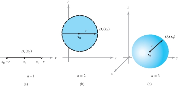
We begin formulating the concept of an open set by defining an open disk. Let \({\bf x}_0 \in {\mathbb R}^n\) and let \(r\) be a positive real number. The open disk (or open ball) of radius \(r\) and center \({\bf x}_0\) is defined to be the set of all points \({\bf x}\) such that \(\| {\bf x}- {\bf x}_0 \| < r\). This set is denoted \(D_r({\bf x}_0)\) and is the set of points \({\bf x}\) in \({\mathbb R}^n\) whose distance from \({\bf x}_0\) is less than \(r\). Notice that we include only those \({\bf x}\) for which strict inequality holds. The disk \(D_r ({\bf x}_0)\) is illustrated in Figure 2.16 for \(n=1,2,3\). For the case \(n=1\) and \(x_0 \in {\mathbb R}\), the open disk \( D_{r}(x_0)\) is the open interval \((x_0 - r, x_0 + r)\), which consists of all numbers \(x \in {\mathbb R}\) strictly between \(x_0 - r\) and \(x_0 + r\). For the case \(n=2, {\bf x}_0 \in {\mathbb R}^2, D_r({\bf x}_0)\) is the “inside” of the disk of radius \(r\) centered at \({\bf x}_0\). For the case \(n=3,{\bf x}_0 \in {\mathbb R}^3, D_r({\bf x}_0)\) is the part strictly “inside” of the ball of radius \(r\) centered at \({\bf x}_0\).
Definition: Open Sets
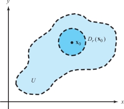
Let \(U\subset {\mathbb R}^n\) (that is, let \(U\) be a subset of \({\mathbb R}^n\)). We call \(U\) an open set when for every point \({\bf x}_0\) in \(U\) there exists some \(r>0\) such that \(D_r({\bf x}_0)\) is contained within \(U\); symbolically, we write \(D_r({\bf x}_0)\subset U\) (see Figure 2.17).
The number \(r>0\) can depend on the point \({\bf x}_0\), and generally \(r\) will shrink as \({\bf x}_0\) gets closer to the “edge” of \(U\). Intuitively speaking, a set \(U\) is open when the “boundary” points of \(U\) do not lie in \(U\). In Figure 2.17, the dashed line is not included in \(U\).
89
We establish the convention that the empty set \(\emptyset\) (the set consisting of no elements) is open.
We have defined an open disk and an open set. From our choice of terms it would seem that an open disk should also be an open set. A little thought shows that this fact requires some proof. The following theorem does this.
Theorem 1
For each \({\bf x}_0 \in {\mathbb R}^n\) and \(r>0,D_r({\bf x}_0)\) is an open set.
proof
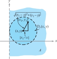
Let \({\bf x} \in D_r({\bf x}_0)\); that is, let \(\| {\bf x} - {\bf x}_0 \| <r\). According to the definition of an open set, we must find an \(s > 0\) such that \(D_s({\bf x}) \subset D_r ({\bf x}_0)\). Referring to Figure 2.18, we see that \(s= r- \| {\bf x} - {\bf x}_0 \|\) is a reasonable choice; note that \(s>0\), but that \(s\) becomes smaller if \({\bf x}\) is nearer the edge of \(D_r({\bf x}_0)\).
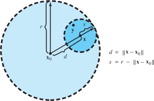
To prove that \(D_s({\bf x})\subset D_r ({\bf x}_0)\), let \({\bf y}\in D_s ({\bf x})\); that is, let \(\| {\bf y} - {\bf x} \| < s\). We want to prove that \({\bf y}\in D_r ({\bf x}_0)\) as well. Proving this, in view of the definition of an \(r\)-disk, entails showing that \(\| {\bf y} - {\bf x}_0\| < r\). This is done by using the triangle inequality for vectors in \({\mathbb R}^n\): \[ \| {\bf y} - {\bf x}_0 \| = \| ({\bf y} - {\bf x}) + ({\bf x} - {\bf x}_0) \| \leq \| {\bf y} - {\bf x} \| + \| {\bf x} - {\bf x}_0 \| < s + \| {\bf x} - {\bf x}_0 \| = r . \]
Hence, \(\| {\bf y} - {\bf x}_0 \| < r\).
The following example illustrates some techniques that are useful in establishing the openness of sets.
90
example 1
Prove that \(A= \{(x,y) \in {\mathbb R}^2 \mid x>0\}\) is an open set.
solution The set is pictured in Figure 2.19.
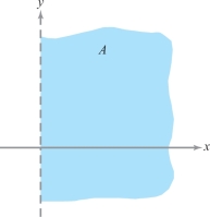
Intuitively, this set is open, because no points on the “boundary,” \(x=0\), are contained in the set. Such an argument will often suffice after one becomes accustomed to the concept of openness. At first, however, we should give details. To prove that \(A\) is open, we show that for every point \((x,y)\in A\) there exists an \(r>0\) such that \(D_r(x,y)\subset A\). If \((x,y)\in A\), then \(x>0\). Choose \(r=x\). If \((x_1,y_1)\in D_r (x,y),\) we have \[ | x_1 - x| = \textstyle\sqrt{(x_1 - x)^2} \leq \textstyle\sqrt{(x_1 - x)^2 + (y_1 - y)^2} < r=x, \] and so \(x_1-x< x\) and \(x - x_1 < x\). The latter inequality implies \(x_1> 0\), that is, \((x_1, y_1)\in A\). Hence \(D_r(x,y)\subset A\), and therefore \(A\) is open (see Figure 2.20).
It is useful to have a special name for an open set containing a given point \({\bf x}\), because this idea arises often in the study of limits and continuity. Thus, by a neighborhood of \({\bf x}\in {\mathbb R}^n\) we merely mean an open set \(U\) containing the point \({\bf x}\). For example, \(D_r ({\bf x}_0)\) is a neighborhood of \({\bf x}_0\) for any \(r>0\). The set \(A\) in Example 1 is a neighborhood of the point \({\bf x}_0 = (3, -10)\).
Boundary
Let us formally introduce the concept of a boundary point, which we alluded to in Example 1.
Definition: Boundary Points
Let \(A\subset {\mathbb R}^n\). A point \({\bf x}\in {\mathbb R}^n\) is called a boundary point of \(A\) if every neighborhood of \({\bf x}\) contains at least one point in \(A\) and at least one point not in \(A\).
In this definition, \({\bf x}\) itself may or may not be in \(A\); if \({\bf x}\in A\), then x is a boundary point if every neighborhood of x contains at least one point not in \(A\) (it already contains a point of \(A\), namely, x). Similarly, if x is not in \(A\), it is a boundary point if every neighborhood of x contains at least one point of \(A\).
We shall be particularly interested in boundary points of open sets. By the definition of an open set, no point of an open set \(A\) can be a boundary point of \(A\). Thus, a point \({\bf x}\) is a boundary point of an open set A if and only if \({\bf x}\) is not in A and every neighborhood of \({\bf x}\) has a nonempty intersection with \(A\).
91
This expresses in precise terms the intuitive idea that a boundary point of \(A\) is a point just on the “edge” of \(A\). In many examples it is perfectly clear what the boundary points are.
example 2
(a) Let \(A=(a,b)\) in \({\mathbb R}\). Then the boundary points of \(A\) consist of the points \(a\) and \(b\). A consideration of Figure 2.21 and the definition will make this clear. [The reader will be asked to prove this in Exercise 28(c).]
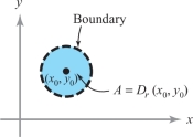
(b) Let \(A=D_r(x_0,y_0)\) be an \(r\)-disk about \((x_0,y_0)\) in the plane. The boundary consists of points \((x,y)\) with \((x-x_0)^2 + (y - y_0)^2 = r^2\) (Figure 2.22).
(c) Let \(A=\{(x,y)\in {\mathbb R}^2 \mid x>0\}\). Then the boundary of \(A\) consists of all points on the \(y\) axis (draw a figure that depicts this).
(d) Let \(A\) be \(D_r({\bf x}_0\)) minus the point \({\bf x}_0\) (a “punctured” disk about \({\bf x}_0\)). Then \({\bf x}_0\) is a boundary point of \(A\).
Limits
We now turn our attention to the concept of a limit. Throughout the following discussions the domain of definition of the function f will be an open set A. We are interested in finding the limit of \(f\) as \({\bf x}\in A\) approaches either a point of \(A\) or a boundary point of \(A\).
You should appreciate the fact that the limit concept is a basic and useful tool for the analysis of functions; it enables us to study derivatives, and hence maxima and minima, asymptotes, improper integrals, and other important features of functions, as well as being useful for infinite series and sequences. We will present a theory of limits for functions of several variables that includes the theory for functions of one variable as a special case.
In one-variable calculus, you have encountered the notion of \({{\rm limit}_{x \rightarrow x_0}}f(x)\,{=}\,l\) for a function \(f\colon\, A \subset {\mathbb R} \rightarrow {\mathbb R}\) from a subset \(A\) of the real numbers to the real numbers. Intuitively, this means that as \(x\) gets closer and closer to \(x_0\), the values \(f(x)\) get closer and closer to (the limiting value) \(l\). To put this intuitive idea on a firm, mathematical foundation, either the “epsilon \((\varepsilon)\) and delta \((\delta)\) method” or the “neighborhood method” is usually introduced. The same is true for functions of several variables. In what follows we develop the neighborhood approach to limits. The epsilon-delta approach is left for optional study at the end of this section.
92
Definition: Limit
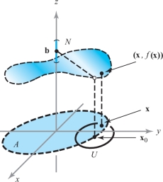
Let \(f\colon\, A\subset {\mathbb R}^n \rightarrow {\mathbb R}^m,\) where \(A\) is an open set. Let \({\bf x}_0\) be in \(A\) or be a boundary point of \(A,\) and let \(N\) be a neighborhood of \({\bf b}\in {\mathbb R}^m\). We say \(f\) is eventually in \(N\) as \({\bf x}\) approaches \({\bf x}_0\) if there exists a neighborhood \(U\) of \({\bf x}_0\) such that \({\bf x}\neq {\bf x}_0,{\bf x}\in U\), and \({\bf x}\in A\) imply \(f({\bf x})\in N\). [The geometric meaning of this assertion is illustrated in Figure 2.23; note that \({\bf x}_0\) need not be in the set \(A,\) so that \(f({\bf x}_0)\) is not necessarily defined.] We say \(f({\bf x})\) approaches b as x approaches \({\bf x}_0\), or, in symbols, \[ \mathop{\hbox{limit}}_{{\bf x}\rightarrow {\bf x}_0} f({\bf x}) = {\bf b}\qquad \hbox{or}\qquad f({\bf x}) \rightarrow {\bf b}\quad \hbox{as}\quad {\bf x} \rightarrow {\bf x}_0, \] when, given any neighborhood \(N\) of b, \(f\) is eventually in \(N\) as x approaches \({\bf x}_0\) [that is, “\(f({\bf x})\) is close to \({\bf b}\) if \({\bf x}\) is close to \({\bf x}_0\)”]. It may be that as \({\bf x}\) approaches \({\bf x}_0\), the values \(f({\bf x})\) do not get close to any particular vector. In this case, we say that \({{\rm limit}_{{\bf x} \rightarrow {\bf x}_0}} f({\bf x})\) does not exist.
Henceforth, whenever we consider the notion \({\rm limit}_{{\bf x} \rightarrow {\bf x}_0} f({\bf x})\), we shall always assume that \({\bf x}_0\) either belongs to some open set on which \(f\) is defined or is on the boundary of such a set.
One reason we insist on \({\bf x}\neq {\bf x}_0\) in the definition of limit will become clear if we remember from one-variable calculus that we want to be able to define the derivative \(f'(x_0)\) of a function \(f\) at a point \(x_0\) by \[ f'(x_0) = {\displaystyle \mathop {{\rm limit}}_{x \,\rightarrow\, x_0}} \frac{f(x)-f(x_0)}{x-x_0} , \] and this expression is not defined at \(x=x_0\).
example 3
(a) This example illustrates a limit that does not exist. Consider the function \(f\colon\, {\mathbb R}\rightarrow {\mathbb R}\) defined by \[ f(x) = \bigg\{ \begin{array}{r@{\qquad}l} 1 & \hbox{if } x>0\\ -1 &\hbox{if } x\leq 0. \end{array} \]
93
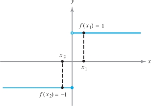
The \({{\rm limit}_{x \rightarrow 0}} f(x)\) does not exist, since there are points \(x_1\) arbitrarily close to 0 with \(f(x_1)= 1\) and also points \(x_2\) arbitrarily close to 0 with \(f(x_2)= -1\); that is, there is no single number that \(f\) is close to when \(x\) is close to 0 (see Figure 2.24). If \(f\) is restricted to the domain \((0, 1)\) or \((-1, 0),\) then the limit does exist. Can you say why?
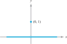
(b) This example illustrates a function whose limit does exist, but whose limiting value does not equal its value at the limiting point. Define \(f\colon\, {\mathbb R}\rightarrow {\mathbb R}\) by \[ f(x) = \bigg\{ \begin{array}{l@{\qquad}l} 0 & \hbox{if }x\neq 0\\ 1 & \hbox{if }x=0. \end{array} \]
It is true that \({{\rm limit}_{x \rightarrow 0}} f(x)=0,\) since for any neighborhood \(U\) of \(0, x\in U\) and \(x \neq 0\) implies that \(f(x)=0\). We see from the graph in Figure 2.25 that \(f\) approaches \(0\) as \(x \rightarrow 0;\) we do not care that \(f\) happens to take on some other value at 0.
example 4
Use the definition to verify that the “obvious” \({{\rm limit}_{\,\,{\bf x} \rightarrow {\bf x}_0}}\, {\bf x} = {\bf x}_0\) holds, where \({\bf x}\) and \({\bf x}_0 \in {\mathbb R}^n\).
solution Let \(f\) be the function defined by \(f({\bf x}) = {\bf x}\), and let \(N\) be any neighborhood of \({\bf x}_0\). We must show that \(f({\bf x})\) is eventually in \(N\) as \({\bf x} \rightarrow {\bf x}_0\). According to the definition, we must find a neighborhood \(U\) of \({\bf x}_0\) with the property that if \({\bf x} \neq {\bf x}_0\) and \({\bf x} \in U\), then \(f({\bf x}) \in N.\) Pick \(U=N\). If \({\bf x} \in U\), then \({\bf x}\in N\); because \({\bf x} = f({\bf x})\), it follows that \(f({\bf x}) \in N\). Thus, we have shown that \({\rm limit}_{{\bf x} \to {\bf x}_0}\) \({\bf x}= {\bf x}_0\). In a similar way, we have \[ {\displaystyle \mathop {{\rm limit}\ }_{(x,y) \rightarrow (x_0, y_0)}} x = x_0, \hbox{etc.} \]
In what follows, you may assume, without proof, the validity of limits from one-variable calculus. For example, \({\rm limit}_{x \rightarrow 1} \sqrt{x} = \sqrt{1} = 1\) and \({\rm limit}_{\theta \rightarrow 0} \sin\, \theta = \sin\, 0 = 0\) may be used.
94
example 5
(This example demonstrates another case in which the limit cannot simply be “read off” from the function.) Find \({\rm limit}_{x\rightarrow 1} g(x)\) where \[ g\colon \,x \mapsto \frac{x-1}{\sqrt{x}-1}. \]
solution This function is graphed in Figure 2.26.
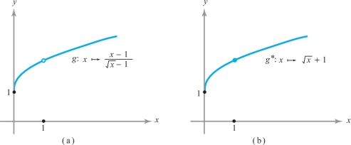
We see that \(g(1)\) is not defined, because division by zero is not defined. However, if we multiply the numerator and denominator of \(g(x)\) by \(\sqrt{x} +1\), we find that for all \(x\) in the domain of \(g\) we have \[ g(x) = \frac{x-1}{\sqrt{x}-1} = \sqrt{x} + 1, \qquad x \neq 1. \]
The expression \(g^*(x) = \sqrt{x} +1\) is defined and takes the value 2 at \(x=1;\) from one-variable calculus, \(g^*(x) \rightarrow 2\) as \(x \rightarrow 1\). But because \(g^*(x) = g(x)\) for all \(x \geq 0, x \neq 1\), we must have as well that \(g(x) \rightarrow 2\) as \(x \rightarrow 1\).
We will consider other examples in two variables shortly.
Properties of Limits
To properly speak of the limit, we should establish that \(f\) can have at most one limit as \({\bf x} \rightarrow {\bf x}_0\). This is intuitively clear and we now state it formally. (See the Internet supplement for the proof.)
Theorem 2 Uniqueness of Limits
\[ \hbox{If}\qquad\displaystyle \mathop{\rm limit}_{{\bf x} \rightarrow {\bf x}_0} f({\bf x}) = {\bf b}_1\qquad\hbox{and}\qquad\displaystyle \mathop{\rm limit}_{{\bf x} \rightarrow {\bf x}_0} f({\bf x}) = {\bf b}_2,\qquad\hbox{then}\qquad{\bf b}_1 \,{=}\,\, {\bf b}_2. \]
To carry out practical computations with limits, we require some rules for limits; for example, that the limit of a sum is the sum of the limits. These rules are summarized in the following theorem (see the Internet supplement for Chapter 2 for the proof).
95
Theorem 3 Properties of Limits
Let \(f\colon\, A\subset {\mathbb R}^n \rightarrow {\mathbb R}^m\), \(g\colon\, A\) \(\subset {\mathbb R}^n \rightarrow {\mathbb R}^m, {\bf x}_0\) be in \(A\) or be a boundary point of \(A, {\bf b} \in {\mathbb R}^m\), and \(c \in {\mathbb R}\); then
- (i) If \({\rm limit}_{{\bf x} \rightarrow {\bf x}_0} f({\bf x}) = {\bf b}\), then \({\rm limit}_{{\bf x} \rightarrow {\bf x}_0} cf({\bf x})= c{\bf b}\), where \(cf\colon\, A \rightarrow {\mathbb R}^m\) is defined by \({\bf x} \mapsto c(f({\bf x}))\).
- (ii) If \({\rm limit}_{{\bf x} \rightarrow {\bf x}_0}f({\bf x}) = {\bf b}_1\) and \({\rm limit}_{{\bf x} \rightarrow {\bf x}_0} g({\bf x}) = {\bf b}_2\), then \({\rm limit}_{{\bf x} \rightarrow {\bf x}_0}\,(f+g)({\bf x}) = {\bf b}_1 + {\bf b}_2\), where \((f+g)\colon\, A \rightarrow {\mathbb R}^m\) is defined by \({\bf x}\mapsto f({\bf x}) + g({\bf x})\).
- (iii) If \(m=1, {\rm limit}_{{\bf x} \rightarrow {\bf x}_0} f({\bf x}) = b_1\), and \({\rm limit}_{{\bf x} \rightarrow {\bf x}_0} g({\bf x}) = b_2\), then \({\rm limit}_{{\bf x} \rightarrow {\bf x}_0}\, (fg)({\bf x}) = b_1b_2\), where \((fg)\colon\, A \rightarrow {\mathbb R}\) is defined by \({\bf x}\mapsto f({\bf x}) g({\bf x})\).
- (iv) If \(m=1\), \({\rm limit}_{{\bf x} \rightarrow {\bf x}_0} f({\bf x}) = b \neq 0\), and \(f({\bf x})\neq 0\) for all \({\bf x}\in A\), then \({\rm limit}_{{\bf x} \rightarrow {\bf x}_0} 1/f({\bf x}) = 1/b\), where \(1/f\colon\, A \rightarrow {\mathbb R}\) is defined by \({\bf x}\mapsto 1/f({\bf x})\).
- (v) If \(f({\bf x}) = (f_1({\bf x}), \ldots, f_m({\bf x}))\), where \(f_i\colon\, A \rightarrow {\mathbb R}\), \(i=1, \ldots, m,\) are the component functions of \(f\), then \({\rm limit}_{{\bf x} \rightarrow {\bf x}_0} f({\bf x}) = {\bf b} = (b_1, \ldots, b_m)\) if and only if \(\,{\rm limit}_{{\bf x} \rightarrow {\bf x}_0} f_i({\bf x}) = b_i\) for each \(i = 1, \ldots, m\).
These results ought to be intuitively clear. For instance, rule (ii) says that if \(f({\bf x})\) is close to \({\bf b}_1\) and \(g({\bf x})\) is close to \({\bf b}_2\) when \({\bf x}\) is close to \({\bf x}_0\), then \(f({\bf x}) + g({\bf x})\) is close to \({\bf b}_1 + {\bf b}_2\) when \({\bf x}\) is close to \({\bf x}_0\). The following example illustrates how this works.
example 6
Let \(f\colon\, {\mathbb R}^2 \rightarrow {\mathbb R}, (x,y) \mapsto x^2 + y^2 +2\). Compute the limit \[ \displaystyle\mathop{\rm limit}_{(x,y) \,\rightarrow\, (0,1)} f(x,y). \]
solution Here \(f\) is the sum of the three functions \((x,y) \mapsto x^2, (x,y) \mapsto y^2\), and \((x,y)\mapsto 2\). The limit of a sum is the sum of the limits, and the limit of a product is the product of the limits (Theorem 3). Hence, using the fact that \({\rm limit}_{(x,y) \rightarrow (x_0,y_0)} x = x_0\) (Example 4), we obtain \[ {\displaystyle \mathop {{\rm limit}\ }_{(x,y) \rightarrow (x_0,y_0)}} x^2 = \left( {\displaystyle \mathop {{{\rm limit}\ } x}_{(x,y) \rightarrow (x_0,y_0)}}\right) \left( {\displaystyle \mathop {{{\rm limit}\ }x}_{(x,y) \rightarrow (x_0,y_0)}}\right) = x^2_0 \] and, using the same reasoning, \({\rm limit}_{(x,y) \rightarrow (x_0,y_0)} y^2=y^2_0\). Consequently, \[ {\displaystyle \mathop {{\rm limit}\ }_{(x,y) \rightarrow (0,1)}} f(x,y) = 0^2 + 1^2 + 2 = 3. \]
Continuous Functions
In single-variable calculus we learned that the idea of a continuous function is based on the intuitive notion of a function whose graph is an unbroken curve; that is, a curve that has no jumps, or the kind of curve that would be traced by a particle in motion or by a moving pencil point that is not lifted from the paper.
96
To perform a detailed analysis of functions, we need concepts more precise than this rather vague notion. An example may clarify these ideas. Consider the specific function \(f\colon\, {\mathbb R}\rightarrow {\mathbb R}\) defined by \(f(x) = -1\) if \(x \leq 0\) and \(f(x) = 1\) if \(x>0\). The graph of \(f\) is shown in Figure 2.27. [The little open circle denotes the fact that the point (0, 1) does not lie on the graph of \(f\).] Clearly, the graph of \(f\) is broken at \(x=0\). Consider also the function \(g\colon\, x \mapsto x^2\). This function is pictured in Figure 2.27. The graph of \(g\) is not broken at any point.
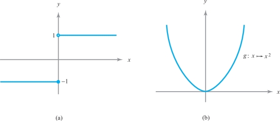
If we examine examples of functions like \(f\), whose graphs are broken at some point \(x_0\), and functions like \(g\), whose graphs are not broken, we see that the principal difference between them is that for a function like \(g\), the values of \(g(x)\) get closer to \(g(x_0)\) as \(x\) gets closer and closer to \(x_0\). The same idea works for functions of several variables. But the notion of closer and closer does not suffice as a mathematical definition; thus, we shall formulate these concepts precisely in terms of limits.
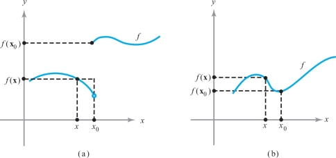
Because the condition \({\rm limit}_{{\bf x} \rightarrow {\bf x}_0} f({\bf x}) = f({\bf x}_0)\) means that \(f({\bf x})\) is close to \(f({\bf x}_0)\) when \({\bf x}\) is close to \({\bf x}_0\), we see that this limit condition does indeed correspond to the requirement that the graph of \(f\) be unbroken (see Figure 2.28, where we illustrate the case \(f\colon\, {\mathbb R}\rightarrow {\mathbb R}\)). The case of several variables is easiest to visualize if we deal with real-valued functions, say \(f\colon\, {\mathbb R}^2\rightarrow {\mathbb R}\). In this case, we can visualize \(f\) by drawing its graph, which consists of all points \((x,y,z)\) in \({\mathbb R}^3\) with \(z=f(x,y)\). The continuity of \(f\) thus means that its graph has no “breaks” in it (see Figure 2.29).
97
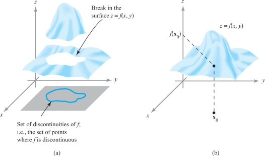
Definition: Continuity
Let \(f\colon\, A \subset {\mathbb R}^n \rightarrow {\mathbb R}^m\) be a given function with domain \(A\). Let \({\bf x}_0 \in A\). We say \(f\) is continuous at \({\bf x}_0\) if and only if \[ {\displaystyle \mathop {{\rm limit}\ }_{{\bf x} \rightarrow {\bf x}_0}} f({\bf x}) = f({\bf x}_0). \]
If we just say that \(f\) is continuous, we shall mean that \(f\) is continuous at each point \({\bf x}_0\) of \(A\). If \(f\) is not continuous at \({\bf x}_0\), we say \(f\) is discontinuous at \({\bf x}_0\). If \(f\) is discontinuous at some point in its domain, we say \(f\) is discontinuous.
example 7
Any polynomial \(p(x) = a_0 + a_1x + \cdots + a_nx^n\) is continuous from \({\mathbb R}\) to \({\mathbb R}\). Indeed, from Theorem 3 and Example 4, \begin{eqnarray*} {\displaystyle \mathop {{\rm limit}\ }_{x \rightarrow x_0}}\big(a_0 + a_1 x + \cdots + a_nx^n\big) &=& {\displaystyle \mathop {{\rm limit}\ }_{x \rightarrow x_0}} a_0 + {\displaystyle \mathop {{\rm limit}\ }_{x \rightarrow x_0}} a_1 x + \cdots + {\displaystyle \mathop {{\rm limit}\ }_{x \rightarrow x_0}} a_nx^n \\ &=& a_0 + a_1 x_0 + \cdots + a_n x^n_0, \end{eqnarray*} because the limit of a product is the product of the limits, which gives \[ {\displaystyle \mathop {{\rm limit}\ }_{x \rightarrow x_0}} x^n = \Big( {\displaystyle \mathop {{\rm limit}\ }_{x \rightarrow x_0}}x\Big)^{n} = x_0^n. \]
example 8
Let \(f\colon\, {\mathbb R}^2 \rightarrow{\mathbb R},f(x,y)=xy\). Then \(f\) is continuous, because, by the limit theorems and Example 4, \[ \mathop {{\rm limit}\ }_{(x,y)\rightarrow(x_0,y_0)} xy=\left( \mathop {{\rm limit}\ }_{(x,y)\rightarrow(x_0,y_0)} x\right)\! \left(\mathop {\rm limit}_{(x,y)\rightarrow(x_0,y_0)} y\right)=x_0y_0. \]
We can see by the same method that any polynomial \(p(x,y)\) [for example, \(p(x,y)=3x^2-6xy^2+y^3\)] in \(x\) and \(y\) is continuous.
98
example 9
The function \(f\colon\, {\mathbb R}^2 \rightarrow {\mathbb R}\) defined by \[ f(x,y)=\bigg\{ \begin{array}{c@{\qquad}l} 1 & \hbox{if } x\leq 0 \hbox{ or } y\leq 0\\[1.2pt] 0 & \hbox{otherwise} \end{array} \] is not continuous at (0, 0) or at any point on the positive \(x\) axis or positive \(y\) axis. Indeed, if \((x_0,y_0)={\bf u}\) is such a point (i.e., \(x_0=0\) and \(y_0\ge 0\), or \(y_0=0\) and \(x_0\ge 0\)) and \(\delta > 0\), there are points \((x,y)\in D_\delta({\bf u})\), a neighborhood of \({\bf u}\), with \(f(x,y)=1\) and other points \((x,y)\in D_\delta({\bf u})\) with \(f(x,y)=0\). Thus, it is not true that \(f(x,y)\rightarrow f(x_0,y_0)=1\) as \((x,y)\rightarrow(x_0,y_0)\).
To prove that specific functions are continuous, we can avail ourselves of the limit theorems (see Theorem 3 and Example 7). If we transcribe those results in terms of continuity, we are led to the following:
Theorem 4 Properties of Continuous Functions
Suppose that \(f\colon\, A\subset{\mathbb R}^n\rightarrow {\mathbb R}^m ,g\colon\, A\subset {\mathbb R}^n\rightarrow {\mathbb R}^m\), and let \(c\) be a real number.
- (i) If \(f\) is continuous at \({\bf x}_0\), so is \(cf\), where \((cf)({\bf x})=c[f({\bf x})]\).
- (ii) If \(f\) and \(g\) are continuous at \({\bf x}_0,\) so is \(f+g\), where the sum of \(f\) and \(g\) is defined by \((f+g)({\bf x}) = f({\bf x})+g({\bf x})\).
- (iii) If \(f\) and \(g\) are continuous at \({\bf x}_0\) and \(m=1\), then the product function \(f\! g\) defined by \((f\! g)({\bf x})=f({\bf x})g({\bf x})\) is continuous at \({\bf x}_0\).
- (iv) If \(f\colon\, A\subset{\mathbb R}^n\rightarrow {\mathbb R}\) is continuous at \({\bf x}_0\) and nowhere zero on \(A\), then the quotient \(1/f\) is continuous at \({\bf x}_0\), where \((1/f)({\bf x})=1/f({\bf x})\).
- (v) If \(f\colon\, A\subset{\mathbb R}^n\rightarrow {\mathbb R}^m\) and \(f({\bf x})=(f_1({\bf x}),\ldots, f_m({\bf x}))\), then \(f\) is continuous at \({\bf x}_0\) if and only if each of the real-valued functions \(f_1, \ldots , f_m\) is continuous at \({\bf x}_0\).
A variant of (iv) is often used: If \(f({\bf x}_0)\not=0\) and \(f\) is continuous, then \(f({\bf x})\not=0\) in a neighborhood of \({\bf x}_0\) and so \(1/f\) is defined in that neighborhood, and \(1/f\) is continuous at \({\bf x}_0\).
example 10
Let \(f\colon\, {\mathbb R}^2 \rightarrow {\mathbb R}^2, (x,y)\mapsto (x^2y,(y+x^3)/(1+x^2))\). Show that \(f\) is continuous.
solution To see this, it is sufficient, by property (v) of Theorem 4, to show that each component is continuous. As we have mentioned, any polynomial in two variables is continuous; thus, the map \((x, y) \mapsto x^2y\) is continuous. Because \(1+x^2\) is continuous and nonzero, by property (iv), we know that \(1/(1+x^2)\) is continuous; hence, \((y+x^3)/(1+x^2)\) is a product of continuous functions, and by (iii) is continuous.
Similar reasoning applies to examples like the function \({\bf c}\colon\, {\mathbb R}\rightarrow {\mathbb R}^3\) given by \({\bf c}(t)= (t^2,1\), \(t^3/(1+t^2))\) to show they are continuous as well.
Composition
99
Next we discuss composition, another basic operation that can be performed on functions. If \(g\) maps \(A\) to \(B\) and \(f\) maps \(B\) to \(C\), the composition of g with \(f\), or of \(f\) on \(g\), denoted by \(f\circ g\), maps \(A\) to \(C\) by sending \({\bf x}\mapsto f(g({\bf x})\)) (see Figure 2.30). For example, \(\sin\, (x^2)\) is the composition of \(x\mapsto x^2\) with \(y\mapsto \sin\, y\).
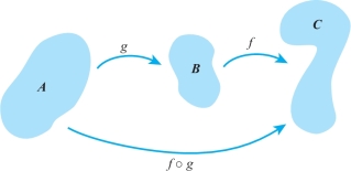
Theorem 5 Continuity of Compositions
Let \(g\colon\, A \subset {\mathbb R}^n\) \(\rightarrow {\mathbb R}^m\) and let \(f\colon\, B \subset {\mathbb R}^m \rightarrow {\mathbb R}^p\). Suppose \(g(A)\subset B,\) so that \(f \circ g\) is defined on \(A\). If \(g\) is continuous at \({\bf x}_0\in A\) and \(f\) is continuous at \({\bf y}_0=g({\bf x}_0),\) then \(f\circ g\) is continuous at \({\bf x}_0\).
The intuition behind this is easy; the formal proof in the Internet supplement follows a similar pattern. Intuitively, we must show that as \({\bf x}\) gets close to \({\bf x}_0,f(g({\bf x}))\) gets close to \(f(g({\bf x}_0))\). But as \({\bf x}\) gets close to \({\bf x}_0, g({\bf x})\) gets close to \(g({\bf x}_0)\) (by continuity of \(g\) at \({\bf x}_0\)); and as \(g({\bf x})\) gets close to \(g({\bf x}_0),f(g({\bf x}))\) gets close to \(f(g({\bf x}_0))\) [by continuity of \(f\) at \(g({\bf x}_0)]\).
example 11
Let \(f(x,y,z)=(x^2+y^2+z^2)^{30}+\sin\, z^3\). Show that \(f\) is continuous.
solution Here we can write \(f\) as a sum of the two functions \((x^2+y^2+z^2)^{30}\) and \(\sin\, z^3\), so it suffices to show that each is continuous. The first is the composite of \((x,y,z)\mapsto (x^2+y^2+z^2)\) with \(u\mapsto u^{30}\), and the second is the composite of \((x,y,z)\mapsto z^3\) with \(u\mapsto \sin\, u\), and so we have continuity by Theorem 5.
Limits in Terms of ε’s and δ’s
We now state a theorem (proved in the Internet supplement for Chapter 2) giving a useful formulation of the notion of limit in terms of epsilons and deltas that is often taken as the definition of limit. This is, in fact, another way of making precise the intuitive statement that “\(f({\bf x})\) is close to b when x is close to \({\bf x}_0\).” To help understand this formulation, the reader should consider it with respect to each of the examples already presented.
Theorem 6
Let \(f\colon\, A\subset {\mathbb R}^n \rightarrow {\mathbb R}^m\) and let \({\bf x}_0\) be in \(A\) or be a boundary point of \(A\). Then \({\rm limit}_{{\bf x}\to {\bf x}_0} f({\bf x})={\bf b}\) if and only if for every number \(\varepsilon > 0\) there is a \(\delta >0\) such that for any \({\bf x}\in A\) satisfying \(0 < \| {\bf x}-{\bf x}_0 \| < \delta\), we have \(\| f({\bf x})-{\bf b} \| < \varepsilon\) (see Figure 2.31).
100
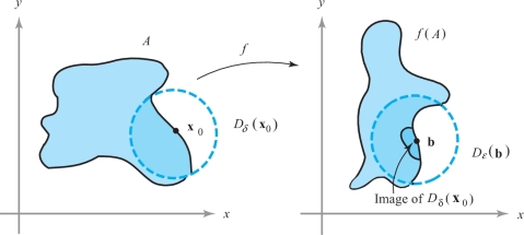
To illustrate the methodology of the epsilon-delta technique in Theorem 6, we consider the following examples.
example 12
Show that \({\rm limit}_{(x,y)\rightarrow (0,0)} x=0\) using the \(\varepsilon\)-\(\delta\) method.
solution Note that if \(\delta > 0, \| (x,y)-(0,0) \| = \sqrt{x^2+ y^2}< \delta\) implies \(|x-0|=|x|=\sqrt{x^2}\leq \sqrt{x^2+y^2} <\delta\). Thus, if \(\| (x,y)-(0,0) \| < \delta\), then \(|x-0|\) is also less than \(\delta\). Given \(\varepsilon >0\), we are required to find a \(\delta >0\) (generally depending on \(\varepsilon\)) with the property that \(0< \| (x,y)-(0,0) \| <\delta\) implies \(|x-0|<\varepsilon\). What are we to pick as our \(\delta\)? From the preceding calculation, we see that if we choose \(\delta =\varepsilon\), then \(\| (x,y)\,{-}\,(0,0) \| <\delta\) implies \(|x\,{-}\,0|\,{<}\,\varepsilon\). This shows that \({\rm limit}_{(x,y)\rightarrow (0,0)} x\,{=}\,0\). Given \(\varepsilon > 0\), we could have also chosen \(\delta=\varepsilon/2\) or \(\varepsilon/3\), but it suffices to find just one \(\delta\) satisfying the requirements of the definition of a limit.
example 13
Consider the function \[ f(x,y)=\frac{\sin\,(x^2+y^2)}{x^2+y^2}. \]
Even though \(f\) is not defined at (0, 0), determine whether \(f(x,y)\) approaches some number as \((x,y)\) approaches (0, 0).
solution From one-variable calculus or L’Hôpital’s rule we know that \[ \mathop {{\rm limit}\ }_{\alpha\rightarrow 0}\frac{\sin\, \alpha}{\alpha}=1. \]
Thus, it is reasonable to guess that \[ \mathop {{\rm limit}\ }_{{\bf v} \to (0,0)}f({\bf v})=\mathop {{\rm limit}\ }_{{\bf v}\rightarrow (0,0)} \frac{\sin\, \| {\bf v} \| ^2}{ \| {\bf v} \| ^2}=1. \]
Indeed, because \({\rm limit}_{\alpha\rightarrow 0}\,(\sin\, \alpha)/\alpha =1\), given \(\varepsilon >0\) we are able to find a \(\delta >0\), with \(0\,{<}\,\delta\,{<}\,1\), such that \(0<|\alpha|<\delta\) implies that \({|(}\sin\, \alpha)/ \alpha-1|<\varepsilon\). If \(0< \| {\bf v} \| <\delta\), then \(0< \|{\bf v} \| ^2<\delta^2<\delta\), and therefore \[ |f({\bf v})-1|=\bigg|\frac{\sin\, \| {\bf v} \|^2}{ \| {\bf v}\|^2}-1\bigg|<\varepsilon. \]
101
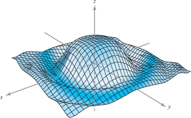
Thus, \({\rm limit}_{{\bf v}\to (0,0)} f({\bf v})=1\). If we plot \([\sin\, (x^2+y^2)]/(x^2+y^2)\) on a computer, we get a graph that is indeed well behaved near (0, 0) (Figure 2.32).
example 14
Show that \[ \mathop {{\rm limit}\ }_{(x,y)\rightarrow (0,0)}\frac{x^2}{\sqrt{x^2+y^2}}=0. \]
solution We must show that \(x^2/\sqrt{x^2+y^2}\) is small when \((x,y)\) is close to the origin. To do this, we use the following inequality: \begin{eqnarray*} 0\leq \frac{x^2}{\sqrt{x^2+y^2}} &\leq& \frac{x^2+y^2}{\sqrt{x^2+y^2}}\qquad \hbox{(because \(y^2\geq 0\))}\\ &=& \textstyle\sqrt{x^2+y^2}.\\[-22pt] \end{eqnarray*}
Given \(\varepsilon >0\), choose \(\delta =\varepsilon\). Then \( \| (x,y)-(0,0) \| = \| (x,y) \| =\sqrt{x^2+y^2}\), and so \(\| (x,y)-(0,0) \| <\delta\) implies that \[ \Bigg|\frac{x^2}{\sqrt{x^2+y^2}}-0\Bigg|=\frac{x^2}{\sqrt{x^2+y^2}}\,\leq \,\textstyle\sqrt{x^2+y^2}= \| (x,y)-(0,0) \| <\delta=\varepsilon. \]
Thus, the conditions of Theorem 6 have been fulfilled and the limit is verified.
example 15
(a) Does \[ \displaystyle \mathop{\rm limit}_{(x,y)\to (0,0)} x^2/(x^2+y^2) \] exist? [See Figure 2.33.]
(b) Prove that [see Figure 2.33] \[ \displaystyle{\mathop{\rm limit}_{(x,y)\,\rightarrow\, (0,0)}}\, \,\frac{2x^2y}{x^2+y^2}=0. \]
102
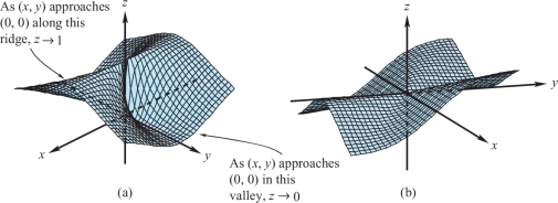
solution (a) If the limit exists, \(x^2/(x^2+y^2)\) should approach a definite value, say \(a\), as \((x,y)\) gets near (0, 0). In particular, if \((x,y)\) approaches zero along any given path, then \(x^2/(x^2+y^2)\) should approach the limiting value \(a\). If \((x,y)\) approaches (0, 0) along the line \(y=0\), the limiting value is clearly 1 (just set \(y=0\) in the preceding expression to get \(x^2/x^2=1\)). If \((x,y)\) approaches (0, 0) along the line \(x=0\), the limiting value is \[ \mathop {\rm lim}_{y\,\rightarrow\, 0}\,\,\frac{0^2}{0^2+y^2}=0 \not=1. \]
Hence, \({\rm limit}_{(x,y)\to (0,0)} x^2/(x^2+y^2)\) does not exist.
(b) Note that \[ \bigg| \frac{2x^2y}{x^2+y^2}\bigg|\leq \bigg|\frac{2x^2y}{x^2}\bigg|=2 |y|. \]
Thus, given \(\varepsilon > 0\), choose \(\delta=\varepsilon/2\); then \(0< \| (x,y)-(0,0) \| =\sqrt{x^2+y^2}<\delta\) implies \(|y|<\delta\), and thus \[ \bigg|\frac{2x^2y}{x^2+y^2}-0\bigg|<2\delta = \varepsilon. \]
Using the \(\varepsilon\)-\(\delta\) notation, we are led to the following reformulation of the definition of continuity.
Theorem 7
Let \(f\colon\, A\subset {\mathbb R}^n\rightarrow {\mathbb R}^m\) be given. Then \(f\) is continuous at \({\bf x}_0\in A\) if and only if for every number \(\varepsilon > 0\) there is a number \(\delta>0\) such that \[ {\bf x}\in A\qquad \hbox{and}\qquad \| {\bf x}-{\bf x}_0 \| <\delta \qquad \hbox{implies} \qquad \| f({\bf x})-f({\bf x}_0) \| <\varepsilon. \]
The proof is almost immediate. Notice that in Theorem 6 we insisted that \(0< \| {\bf x}-{\bf x}_0 \| \); that is, \({\bf x}\not={\bf x}_0\). That is not imposed here; indeed, the conclusion of Theorem 7 is certainly valid when \({\bf x}={\bf x}_0\), and so there is no need to exclude this case. Here we do care about the value of \(f\) at \({\bf x}_0\); we want \(f\) at nearby points to be close to this value.